Bayesian Plate models with PyTensor - Part 1

Probabilistic models with repetitive structures: how to implement them in Python.

Bayesian network are at the base of many machine learning models. They let you model the physical world in a probabilistic way.

The probability distributions that we construct typically contain structures that repeat; e.g over

• Spatial locations
• Time steps
• Users
• Items

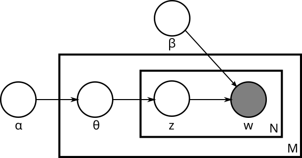
Figure Figure 1 shows plate notation for a Latent Dirichlet Allocation model. The model is used to find topics in a collection of documents. \(M\) refers to the number of documents, while \(N_i\) refers to the number of words in document \(i\).

Figure 1: LDA in plate noteation, created by Bkkbrad for Wikimedia under Creative Commons Attribution-Share Alike

The re-occurring bits of the probability distribution can be neatly summarised in plate notation. Let’s refer to such models as plate models.

In this series of posts, I show how to implement plate structures in Python with PyTensor. Let it be a blueprint for implementing other plate models in Python.

AR(m)

As example we take this time series model:

\[ \begin{align*} y_t &= \rho_1 y_{t-1} + \rho_2 y_{t-2} + \ldots + \rho_{m} y_{t-m} \varepsilon_t, \quad \varepsilon_t \sim \mathcal{N}(0, \sigma^2) \,. \end{align*} \]

This is the autoregressive model of order m, AR(m).

The inference process for AR(n) with PyMC, is described here.

PyTensor is used by PyMC to build computation graphs for generative models. This posts goes in-depth on the construction of computation graphs with PyTensor. A good understanding of PyTensor allows you to build more complex models.

Plate models are very powerfull, but they require loops for implementation. Loops are especially tricky to implement in computation graphs. That’s why I have split the post in two parts:

• Part 1: introduction to PyTensor
• Part 2: building loops into the computation graph

PyTensor basics

PyTensor is a symbolic computation library for Python. It is similar to Theano and TensorFlow, in that it builds a computation graph.

Let’s start building a computation graph for this model

Computation graph

import pytensor
import pytensor.tensor as pt
from pytensor import pp

# Define the constants
lags = pt.iscalar('lags')
n = pt.iscalar('n')
n_steps = n - lags

In PyTensor, all variables are symbolic with a pre-defined type. We have now defined a small graph, that can be visualized with pretty print:

pp(n_steps)

'(n - lags)'

The graph can be evaluated to return an array.

n_steps.eval({n: 10, lags: 2})

array(8, dtype=int32)

Besides scalars, we can define vectors and matrices of type integer or float:

y = pt.fvector('y')
y_init = pt.fvector('y_init')
y_lag = pt.fvector('y_lag')
rho = pt.fvector('rho')

• The time series y is a vector of length n and type float
• The initial values y_init form a vector of length lags and type float
• The lagging values y_init form a vector of length lags and type float
• The autoregressive coefficients rho are a vector of length lags and type float

Functions

Given y_lag and rho, we can compute the next value of the time series y_next. We can build a computation graph for that and turn it into a function

from pytensor.tensor.random.utils import RandomStream
srng = RandomStream(seed=234)
ε = srng.normal(0, 1, size=(1,))
y_next = y_lag.dot(rho) + ε

ε is a node in the graph that produces random numbers from a normal distribution.

ε.eval()

array([-0.53217654])

We can compile this part of the computation graph into a function.

ar_next = pytensor.function([y_lag, rho], y_next)

All that pytensor.function needs are the input nodes and the output nodes.

Let’s evaluate the new function:

import numpy as np
for i in range(3):
  print(ar_next(np.array([1., 2.], dtype=np.float32), np.array([0.5, 0.3], dtype=np.float32)))

[0.50094772]
[1.53177901]
[2.71876207]

The dot-product hides a loop over the lags.

For the AR(n) model we need to unroll the computation graph over time. This time we can’t escape a loop.

In part 2, we are going to build computation graphs with loops.